Benchmarking Solana gRPC stability

Stable gRPC connections are vital for fast and stable Solana update ingestion. Benchmarks used to compare these data services are highly generalized and do not help in measuring several important data points.

The overgeneralized benchmark tool

Almost all modern published benchmarks are performed using Geyserbench (or a fork of this tool). This is a generalized tool that can put several services head-to-head and let them compete in a first-to-arrive competition. Whichever service delivers the most messages fast wins and (often) gets a p50 measurement of 0.00ms. These measurements are almost exclusively done with TX subscriptions, crucially skipping the often more important streaming techniques (like account streaming).

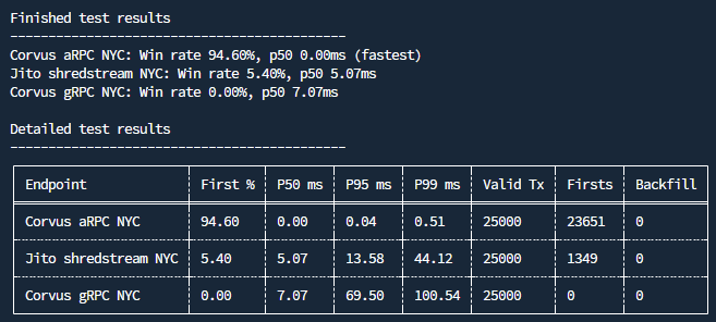
An example benchmark performed using the generic Geyserbench tool

Using this tool to get a general grasp of performance between two services is useful, but it hides the answer to several questions, including:

How stable are the provided services? How much latency is imposed before and after the geyser plugin emits the update messages?
How does every service provider perform on validators that are close-by, or further away? Is there a local geographical advantage that is cancelled out in the noise of all other slots?
When does the losing service start winning? Why can it still beat the winning service sometimes?

On top of this, the Geyserbench tool hardly allows for detailed post-analysis on the raw data generated by the benchmarks. Benchmark results are immediately discarded after benchmark completion, making it hard to identify issues in the raw data.

Explaining observed latency

In order to help gRPC providers identify issues in their own pipeline, I built a tool that can find the hidden answers to the questions outlined in The overgeneralized benchmark tool. This tool measures the reported created_at timestamp (some providers unfortunately hide this measurement) and uses it to calculate when an update was emitted by the gRPC geyser pessimistically (giving the benefit of the doubt to the gRPC geyser). More importantly, this tool does not require access to the service backend to do its measurements. To do this, I calibrate the difference between created_at - latency_to_endpoint to our clock, making it possible to determine if an update has been in flight for too long. We can even notice the Linux clock drifting at this measurement granularity (yes, the Linux clock drifts, but it usually corrects itself by speeding up and slowing down the clock).

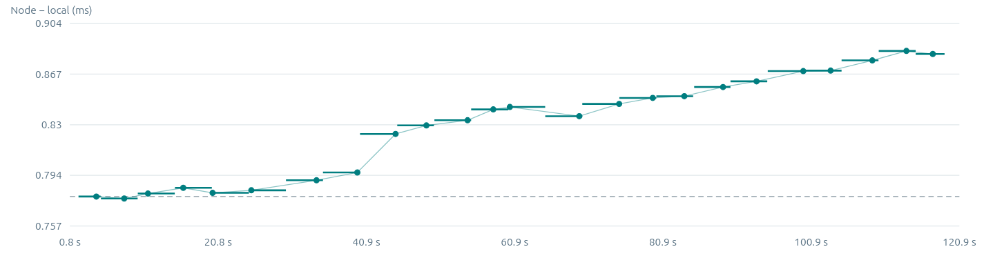
Linux clock drifting between our benchmark machine and the benchmarked server

After compensating for latency and the ever-changing Linux clock, we finally get a raw view at the latency variance that is imposed after gRPC geyser emission. This data looks very different for different types of nodes and it helps to judge which nodes are (likely) oversold and less competitive. I call all excess latency observed after geyser update emission "unexplained latency". Below, you can compare the unexplained latency between an unstable public gRPC provider and a stable (more private) one.

A provider with high unexplained latency (unstable)

A provider with low unexplained latency (stable)

Since we are now able to explain if provider gRPC latency is explained by congestive issues or simply a slow(er) node, we are in a position now to start calling out providers for being congested or for having bad shreds (depending on the unexplained latency benchmark results). This helps us estimate all sorts of properties for competitive node providers, including the quality of their shreds. Using this information, it is possible to make significantly more informed decisions. While this is not the only latency factor in a service, it is often the most dominant reason for an oversold node to be losing against other nodes.

Other advantages

While it is harder to show other advantages of this tool without exposing trading edge, this tool brings much more granular tooling into my kit, including:

The ability to pit two benchmarked targets against eachother in the context of a larger benchmark. Head-to-head latency between two providers might get lost in a benchmark of five providers.
Identify and attribute lag spikes to different causes, like shred delivery / congestion issues for the node provider.
Full replayability and filtering of any past benchmark that has not been discarded, all updates and timing are available, post-analysis was never easier.
Investigate episodes of instability that are automatically flagged in a section that compares global instability across the benchmark and flags anomalies.
The ability to view every latency percentile between benchmarked providers, so you actually know how often your service provider beats a competitor.
More advantages that I cannot reveal. They might give up my edge ;)

Large traffic spike shows median traffic arriving delayed on a benchmarked service provider. This elevated latency window took 3.5 seconds

All of this research was conducted with limited insights into the benchmarked services. Several of the service providers I contacted about their internal issues originally waived these as non-issues. Bringing these detailed reports made them change their stance and helped in convincing them that their data feed quality was poor, as well as debug where the latency was being imposed. Hopefully, this article helps you come prepared in your future instability reports!